Previous Up Next

2  Tree Automata, Clauses

Automata on finite words are a very classical data structure to represent sets of words—possibly infinite sets. Not all sets of words can be described this way; such special sets are called regular languages. Regular languages are reasonably expressive, and all the basic operations are computable on them: testing for membership, for vacuity, computing unions, intersections, complements notably.

An example of automaton is shown below. This is just a directed graph. Vertices are traditionally called states, and edges are called transitions. Two other components are needed. First, we need an initial state: in the example, we assume this is qinit. Second, we need final states. The convention is that final states are circled; here, the only final state is qinit.


Let us play a game. You start at the initial state qinit, then you must follow some transitions (whichever you wish, you may even repeat the same transition as long as you wish), until you reach a final state. While traveling around, collect the letters that label the transitions: this gives you a sequence of letters, i.e., a word. (One exception, though: the є symbols means “no letter”, and you should just go through the corresponding transition without collecting any letter at all.) The fact that you reached the final state is how you decide that the automaton recognized the word.

For example, starting from qinit, you may go up the a transition, then come back along the є transition. Since you've reached a final state, namely qinit (which is both initial and final), the word a is recognized by the automaton. Or you may have decided to start from qinit, go up the a transition, turn once inside the b loop, then come back through the є-transition: the word ab is recognized. In fact, you might have looped as many times as you wished, so any word abn, n in |N, is recognized, too.

There is no need to stop when you reach a final state. For example, we may travel along a, then b twice, then along є, then again along a, then b three times, then є, showing that ab2ab3 is recognized. While we are at it, since qinit is already final, the empty word (with no letter) is also recognized. We write є for the empty word, as is traditional.

To wrap up the example, the above automaton recognizes exactly the language (a b*)*, that is the set of all words on the alphabet {a,b} which are concatenations of words a bn, n in |N. It turns out that this is just the set of words that, if non-empty, start with a.

Alternatively, we can describe this same set of words as a set of Horn clauses, i.e., as a very simple Prolog program. To this end, create a fresh predicate symbol q for each state q. The meaning of q(t) is that the word t should be recognized at q, i.e., there is a trip along the transitions in the automaton, starting from the initial state, and ending exactly on the state q, along which the letters collected form the word t. We also encode words as terms: є will be a constant denoting the empty word, and we add each letter ℓ at the end of word t by writing the term ℓ (t); this means in particular that each letter is now viewed as a unary function symbol. The automaton above then gets described as a Prolog program with one clause for each transition, plus one to say that the empty word is recognized at the initial state:
qinit (є)   q1 (a (X)) :- qinit (X)
q1 (b (X)) :- q1 (X)   qinit (X) :- q1 (X)
You may ask Prolog whether the word ab2 is recognized at qinit by submitting the query
?qinit (b (b (a (є))))
and it will answer “yes”. Prolog will also answer the query
?qinit (b (b (a (b (є)))))
by “no”, meaning that bab2 is not in the language.

Prolog, as a notation, is fine, as we shall see. Prolog, as a tool to check properties, is ill-suited: on the more complex clauses we shall encounter below, Prolog would loop infinitely in general; h1 on the other hand is meant to return, always, on its input clauses.

The notion of automata, on words, can be generalized to automata on first-order terms, a.k.a., tree automata. These are very similar structures, except they recognize sets of ground terms. The automaton of Figure 1, to take an example, recognizes the set of all lists of even natural numbers at state qlisteven. To be precise, it recognizes the set of all terms cons (t1, cons (t2, …, cons (tn, nil) …)), where each ti is of the form Sni (O), ni even. Note that the transition O (up left) starts from no state, while the transition cons (_, _) (middle) starts from a pair of states, qeven and qlisteven.


Figure 1: Recognizing the lists of even natural numbers


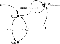
To define the semantics of tree automata, the simplest is just to describe their translation to Horn clauses. Each transition again gives rise to exactly one clause:
qeven (O) qeven (S (X)) :- qodd (X) qodd (S (X)) :- qeven (X)
  qlisteven (cons (X, Y)) :- qeven (X), qlisteven (Y) qlisteven (nil)
There is no need to define initial states in tree automata; e.g., O is recognized at qeven, using the transition qeven (O), of arity 0.

In general, a tree automaton is any finite set S of clauses of the form
  P (f (X1, …, Xn)) :- P1 (X1), …, Pn (Xn)     (1)
where X1, ..., Xn are pairwise distinct variables. When n=0, we retrieve initial clauses such as qeven (O). When n is restricted to be at most 1, tree automata are just ordinary, word automata (without є-transitions).

A set of ground terms is called regular if and only if it is exactly the set of terms t such that t is recognized at P in some tree automaton S (i.e., such that P (t) follows logically from the clauses in S).

The format of clauses (1) is very particular. First, clauses (1) are definite clauses. Formally, definite clause are implications of the form
  P (t) :- P1 (t1), …, Pn (tn)     (2)
where P (t), P1 (t1), ..., Pn (tn) is an unordered set of atoms. (An atom is just a predicate P applied to some term t; read “P holds of t”, or “t is recognized at P”.) If n=0, this is called a fact, and is often written just P (t).

Any set S of definite clauses has a least Herbrand model. A Herbrand model is just a collection of ground atoms P (t). The least Herbrand model H (S) of S can be described as follows. First, it contains all ground instances of the facts in S. Then, while there is a ground instance P (t σ) :- P1 (t1 σ), …, Pn (tn σ) of a clause P (t) :- P1 (t1), …, Pn (tn) in S, and P1 (t1 σ), ..., Pn (tn σ) are in H (S), then add P (t σ) to H (S). This procedure does not terminate in general, but enumerates H (S).

In particular, any tree automaton has a least Herbrand model. It turns out that the ground atom P (t) is in the least Herbrand model H (S) if and only if t is recognized at P in the tree automaton S. Therefore, we may generalize the notion of a term t being recognized at some predicate P in any set of definite clauses, by requiring that P (t) is in H (S).

A goal clause is an implication of the form
  false :- P1 (t1), …, Pn (tn)     (3)
where false is meant to denote false. A Horn clause is a definite or a goal clause. We shall also write P (t) instead of P (t) :- when n=0, and false instead of false :- .

Not any set S of Horn clauses has a model. If it has one, that is, if S is satisfiable, then it again has a least Herbrand model H (S). Again, we say that t is recognized at P in S if and only if P (t) is in H (S).

Then it can be shown that the ground term t is recognized at P in the set S of definite clauses if and only if S plus the goal clause false :- P (t) is unsatisfiable (i.e., not satisfiable); that P is empty in S, i.e., that P recognizes no term in S, if and only if S plus the clause false :- P (X) is unsatisfiable, where X is a variable. And there are automated means, called automated theorem provers, to check the unsatisfiability of clause sets. Unfortunately, they do not always terminate. The h1 tool always terminates, but only deals with so-called H1 clauses [2002  (Nielson et al.)].

We have said above that tree automata clauses (1) were very particular, because they were definite clauses, and in particular they always have a least Herbrand model. They are also particular in that the head (the atom at the left of :- ) is restricted to be of the form P (t) with t itself of the form f (X1, …, Xn), where X1, ..., Xn must be distinct variables; and in that there is no function symbol at all in the body (the set of atoms at the right of :- ).

If you do not restrict the form of Horn clauses (2) and (3), then any prover that operates on them is forced to relinquish either termination, soundness, or completeness. This is because the satisfiability of Horn clauses is undecidable [1996  (Devienne et al.)]. Most automated theorem provers in existence are sound, i.e., if they deduce a contradiction from S then S is unsatisfiable, and complete, i.e., if S is unsatisfiable then they can derive a contradiction from S. Therefore they have to fail to terminate sometimes. On the other hand, h1 is complete and terminates, but is only sound on the subset of so-called H1-clauses.

The H1-clauses are exactly the Horn clauses, except that definite clauses (1) are restricted to have a head of the form P (X), where X is a variable, or P (f (X1, …, Xn)), where X1, ..., Xn are distinct variables. While this is not the definition [2002  (Nielson et al.)], this is equivalent to it, see [2005  (Goubault-Larrecq)].

On general Horn clauses, h1 applies an abstraction function which makes it still a terminating and complete prover, but one which is unsound in general. So you might want to see h1 as a counter-model finder rather than a prover. In some cases, though, h1 produces unsound “proofs” that may be indicative of actual proofs.

Remember that h1 is sound, complete, and terminating on H1 clauses. Note that automata clauses are a special case of H1 clauses. In fact, when h1 terminates, starting from a set S of H1 clauses, there are two possible outcomes: In the latter case, h1 also produces a model of S, in the form of an alternating tree automaton, i.e., a set of clauses of the form
  P (f (X1, …, Xn)) :- B1 (X1), …, Bn (Xn)     (4)
where Bi (Xi) is a block, i.e., a list of atoms Pi1 (Xi), …, Pini (Xi). Note that tree automata clauses are a special case of alternating tree automata clauses (take ni=1 for each i), while alternating tree automata clauses are special H1 clauses (with no function symbol in the body, the head is of the form P (f (X1, …, Xn)) and not P (X), and every variable free in the body is among X1, …, Xn).

From a theoretician's perspective, this means that H1 clauses are not more expressive than alternating tree automata clauses. And it is well-known that alternating tree automata are not more expressive than plain tree automata: the languages defined by satisfiable H1 clause sets are just, again, the regular tree languages. However, H1 offers considerably more freedom in describing such languages than just using tree automata, because of the general form of H1 clauses.

The paper that introduced H1 is [2002  (Nielson et al.)]. For some background theory on the way h1 works, deciding H1 and converting H1 clause sets to tree automata by resolution techniques, and abstracting general clause sets to H1 clause sets, see [2005  (Goubault-Larrecq)].


Previous Up Next